Building

Building on information presented in my previous post, this articles describes how bagging and boosted can be used to build a classification model. The data is available from Kaggle, and represents the financial transactions from two hundred thousand individuals (each with 800 features).

Using this dataset, I set about building a loan-default model. The overall pipeline for this project was split into a few stages, all of which are described below.

1. Environment Setup
   • MySQL.
   • Numpy
   • Pandas.
   • Scikit-Learn.
2. Reading MySQL data.
3. Preprocessing
   • Dealing with missing values.
   • Dealing with categorical variables.
4. Model Training
   • Gradient Boosting.
5. Model Testing.

Environment Setup

Python packages were first loaded to ensure the data can be accessed and manipulated. Pandas is perfect for this task as it helps data scientists organise and manipulate information. Other packages were also loaded for later data analysis, included:

• matplotlib - used for plotting.
• seaboard  - used for graph formatting.
• scipy - used for statistical analysis.
• pymysql - used for import data from MySQL.
• sklearn - used for model training and testing.

%matplotlib inline

%config InlineBackend.figure_format='retina'
from __future__ import division
from itertools import combinations
import string
import matplotlib.pyplot as plt
import numpy as np
import pandas as pd
import scipy as sp
import pymysql
import seaborn as sns
sns.set()
plt.rcParams['figure.figsize'] = (12, 8)
sns.set_style("darkgrid")
sns.set_context("poster", font_scale=1.3)

Reading data

Having set up the python environment, I set out to read data from MySQL using  pymysql and the following code:

con = pymysql.connect(host='127.0.0.1',port=3306, user='root', passwd='xxxx', db='DB_Name')
cur = con.cursor()
Borrowers_DataFrame = pd.read_sql("SELECT * FROM BORROWERS_All", con=con)
print(' Data Frame successfully imported.')
con.close()

Great news, we can now access the data in Python. Lets start modelling!

Preprocessing Data

But wait…The quality of information is key to determine how well a machine learning algorithm will perform. It where therefore vital to examine data before it's used in a machine learning algorithm, all of which is discussed in this section.

Dealing with Missing Values - Imputing Data

The removal of missing samples is not feasible in many examples because we might lose too many observations. In this case it is best to use mean imputation to estimate the missing values from the remaining data. This simply implies that NaN values are replaced by the average value for each feature, and scikit-learn's Imputer class allowed me to complete this task.

from sklearn.preprocessing import Imputer
imr = Imputer(missing_values='NaN', strategy='mean', axis=0)
imr = imr.fit(Borrowers_DataFrame) imputed_data = imr.transform(Borrowers_DataFrame.values)

Dealing with Categorical Variables - One Hot Encoding

Nominal and ordinal categorical variables are common features in real-world datasets. Simply put, ordinal refers to categorical variables that can be sorted (e.g. t-shirt size), whilst nominal features cannot be differentiated by size (e.g. dog breed). Only nominal features were included in the Kaggle dataset, so I simply needed to map each string to an integer value.

A common technique for this task is one-hot encoding. This approach creates a new dummy feature for each unique value, where I split a feature of three countries into separate columns: (e.g. Ireland, USA, and UK). Binary values can then be used to indicate the particular country of a sample, where, for example, an Irish sample can be encoded as Irish=1, USA=0, UK=0.

To perform this transformation, I used the OneHotEncoder from the scikit-learn.preprocessing module, which is implemented using the get_dummies command:

from sklearn.preprocessing import OneHotEncoder
OHE_Imputed_DF_Sampled = pd.get_dummies(imputed_data)

Gradient Boosting Model

Step 1: Quick Fit

A Gradient Boosted Model (GBM) was used to develop the initial classification model. GBMs are often prone to overfitting in the absence of parameter tuning, so particular attention was paid to the optimization of hyperparameters. Before I focused on the stage of model tuning, I first implemented a simple GBM ensemble using the following code.

from sklearn.ensemble import GradientBoostingClassifier
estimator = ensemble.GradientBoostingRegressor(n_estimators=200, max_depth=3)
estimator.fit(X_train, Y_train)
result = estimator.predict(X_test)
result = np.expm1(result)

Step 2: Test-Training Split

The next step focuses on segmentation of the complete dataset into a separate training and test set (80% for training, and 20% for testing) using the following code:

from sklearn.utils import shuffle
from sklearn.cross_validation import train_test_split
X, y = OHE_Imputed_DF_Sampled.iloc[:, 1:], OHE_Imputed_DF_Sampled.iloc[:,0]
X, y = shuffle(X, y, random_state=1)
# We do this to shuffle the data that is used each time.
X_train, X_test, y_train, y_test = train_test_split(X, y, test_size=0.2, random_state=0)

Step 3: Parameter Tuning

Finally, I focused on tuning the GBM’s parameters to optimize model performance. For this, I used GrigSearchCV to return a summary of: (1) model's accuracy scores and (2) the optimal parameters.

from sklearn.grid_search import GridSearchCV
from sklearn.cross_validation import cross_val_score

param_grid = {'learning_rate': [0.2],
              'max_depth': [10, 15, 20],
              'min_samples_leaf': [10, 20],
              'subsample': [0.7, 0.8]}
estimator = GradientBoostingClassifier(loss="deviance",
                                     random_state=0,
                                     n_estimators=10)
gs_cv = GridSearchCV(estimator,
                     param_grid,
                     scoring='accuracy',
                     cv=10,
                     n_jobs=-1)
scores = cross_val_score(gs_cv, X_train, y_train, scoring='accuracy', cv=5)
print('CV accuracy: %.3f +/- %.3f' % (np.mean(scores), np.std(scores)))
gs_cv.fit(X_train, y_train)

print('Best Grid Search CV accuracy score: %s' % gs_cv.best_score_)
print('Optimal Depth: %s' % gs_cv.best_estimator_.max_depth)
gs_cv.best_params_

CV accuracy: 0.724 +/- 0.012
Best Grid Search CV accuracy score: 0.739256976545
Optimal Depth: 15 
{'learning_rate': 0.2,
 'max_depth': 15,
 'min_samples_leaf': 10,
 'subsample': 0.8}

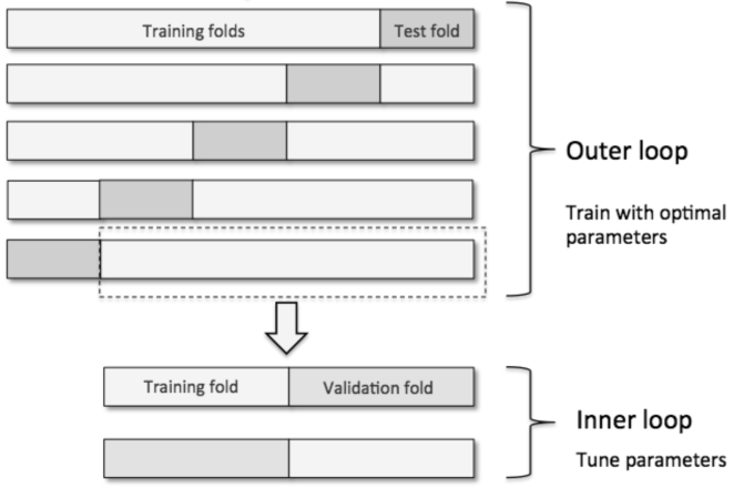
The above code combines k-fold cross-validation with grid search to fine-tune machine learning model performance. More specifically, nested cross-validation first splits the data into training and test folds in an outer k-fold loop before an inner loop is used to fine-tune the model's parameters. A test fold (from the outer loop) is finally used to evaluate the model performance, leading to a true error for the estimate that is almost unbiased relative to the test set. Raschka provides an excellent summary of this concept in there following figure, where there are five outer and two inner folds (i.e. 5x2 cross-validation).

Tuning the number of estimators with Validation Curves

The GBM performance will always improve as the number of estimators is increased. Overfitting can, however, start to become an issue with more ensembles, which is why validation curves are used to visualise and improve model performance.  These are constructed by plotting the error on both the training and validation sets as a function of the estimators used, where the following code generates such a curve.

from sklearn.learning_curve import validation_curve

param_range = range(1,50,1)
clf = GradientBoostingClassifier(learning_rate = 0.2,
 max_depth = 15,
 min_samples_leaf = 10,
 subsample = 0.8)
train_scores, test_scores = validation_curve(
 estimator=clf,
 X=X_train,
 y=y_train,
 param_name='n_estimators',
 param_range=param_range,
 cv=4,
 n_jobs=-1)

train_mean = np.mean(train_scores, axis=1)
train_std = np.std(train_scores, axis=1)
test_mean = np.mean(test_scores, axis=1)
test_std = np.std(test_scores, axis=1)


plt.style.use('ggplot')
plt.plot(param_range, train_mean,
         color='blue', marker='o',
         markersize=5, label='training accuracy')

plt.fill_between(param_range, train_mean + train_std,
                 train_mean - train_std, alpha=0.35,
                 color='blue')

plt.plot(param_range, test_mean,
         color='green', linestyle='--',
         marker='s', markersize=5,
         label='validation accuracy')

plt.fill_between(param_range,
                 test_mean + test_std,
                 test_mean - test_std,
                 alpha=0.10, color='green')

plt.grid()
plt.legend(loc='lower right', fontsize = 20)
plt.title('Error vs. Number of Estimators', fontsize=20)
plt.xlabel('Number of Estimator', fontsize = 20)
plt.ylabel('Accuracy', fontsize = 20)
plt.xticks(fontsize = 18)
plt.yticks(fontsize = 18)
plt.ylim([0.55, 1.01])
plt.tight_layout()
plt.show()

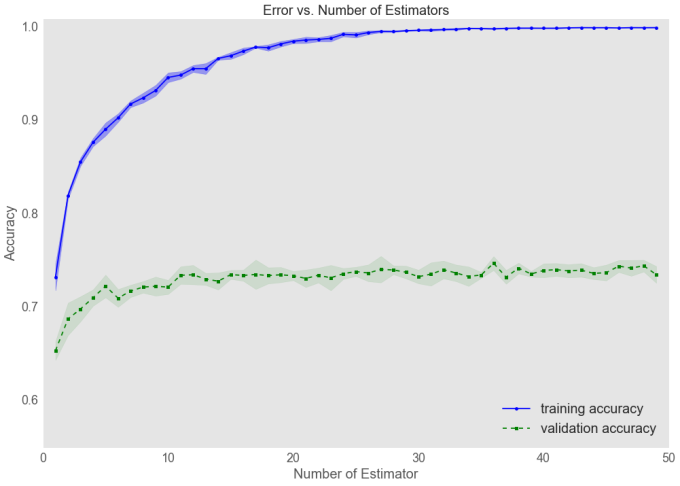
This validation_curve function uses stratified k-fold cross-validation to estimate the performance of classification models . Inside, I specified the parameter that we wanted to evaluate, in this case is the number of estimators (n_estimators). The resulting plot indicates that the model begins to overfit as the number of estimates increases beyond approximately 10 and moving forward, I set n_estimators to 8, rather than 50 to avoid overfitting.

ROC Curve

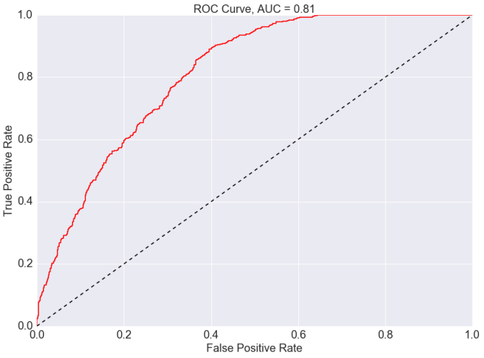
Finally, I plot a Receiver Operating Curve (ROC) to access the performance of the GBM with respect to the false positive and true positive predictions. A perfect classifier would fall into the top-left corner of the graph, where the true positive rate would be 1 and the false positive rate would be 0. I can also compute the area under the curve (AUC) which represents the performance of the GBM. The plot shows that I have been able to achieve reasonable high performance from the GBM, and yields additional insights into the classifier's performance when dealing with imbalanced samples.

sns.set_style("darkgrid")

Defaulted_RF_Prediction = gs_cv.predict_proba(X_test)
fpr, tpr, _ = roc_curve(y_test, Defaulted_RF_Prediction[:,1])
#fpr, tpr, thresh = roc_curve(y_test, Defaulted_RF_Prediction[:,1], pos_label=1,sample_weight=weights)
ROC_DF = pd.DataFrame(dict(fpr=fpr, tpr=tpr))

plt.figure(2)
title = 'ROC Curve, AUC = {}'.format(round(auc(fpr, tpr),2))
plt.title(title, fontsize = 20)

plt.plot(fpr, tpr,'r')
plt.plot([0, 1], [0, 1], 'k--')
plt.xticks(fontsize = 20)
plt.yticks(fontsize = 20)
plt.xlabel('False Positive Rate', fontsize = 20)
plt.ylabel('True Positive Rate', fontsize = 20)
plt.show()

Summary

This post briefly runs through the steps required to develop a Gradient Boosted Model in scikit-learn. With further feature extraction, additional improvements can be made to improve performance. The initial results are promising but, more importantly, the development of this simple boosted models was a fun way to spend an evening!